

Neural Networks along with deep learning provide a solution to image recognition, speech recognition, and natural language processing problems. The Introduction video on TensorFlow and Deep Learning gave an overview of how a neural network and deep learning help on a Classification Problem to Classify hand-written images and how it was actually done with TensorFlow got cleared. Again after viewing the following video to understand well.
There are some basic processes in neural networks are followed in any kind of models. They are,
(i) Initialization,
(ii) Building Model,
(iii) Loss Functions,
(iv) Model Evaluation
All these steps being implemented with the following TensorFlow code,
#Initialization
import tensorflow as tf
X = tf.placeholder(tf.float32, [None, 28, 28, 1])
W = tf.Variable(tf.zeros([784, 10]))
b = tf.Variable(tf.zeros[10])
init = tf.initialize_all_variables()

#The Model
Y = tf.nn.softmax(tf.matmul(tf.reshape(X, [-1, 784]), W) + b)

#Placeholder for Correct Answer
Y_ = tf.placeholder(tf.float32, [None, 10])

#Loss Function
cross_entropy = -tf.reduce_sum(Y_ * tf.log(Y))

# Model Evaluation
is_correct = tf.equal(tf.argmax(Y, 1), tf.argmax(Y_, 1))
accuracy = tf.reduce_mean(tf.cast(iscorrect, tf.float32))
Initialization:
The initialization step basically involves Placeholder and Variable declaration. A placeholder is used for input data and variable stores the state of the output. We use tf.variable for trainable variables such as Weights(W) and Biases(b) for the model. tf.placeholder is used to feed the actual training images. The weight(W) is a TensorFlow Variable which has the dimension of 784 input features and 10 outputs (So 784 x 10 matrix) and bias(b) being a 10-dimensional vector.
Building Model:
Activation Function:
The Wikipedia definition – In computational networks, activation function of a node defines the output of that node given an input or sets of inputs.
Here model is the Sigmoid function,
y = tf.matmul(x, W) + b
The reshape command makes the 28 * 28 = 784 pixels to flatten as a single vector in a single line.
Loss Function:
The function actually minimizes the loss of training images which could improve the overall performance of the scenario. So, here the loss function is a cross-entropy between the target and the softmax activation function applied to the model’s prediction. tf.reduce_sum takes the average over the sums of all classes.
Training the Model:
The Optimizer in training step actually does the job of minimizing the error function/loss function. We modify the weights and biases so as to minimize to point a new direction in the training process will give better results, is known as Gradient Descent and here is the training loop,
sess = tf.session()
sess.run(init)

for i in range(1000):
# Load batch of images & correct answers
batch_X, batch_Y = mnist.train.next_batch(100)
train_data = { X: batch_X, Y_: batch_Y }
sess.run(train_step, feed_dict=train_data)
# Success
a, c = sess.run([accuracy, cross_entropy], feed_dict=train_data)
When the tf. some command runs, it won’t give any values instead it build some Computational graphs in memory. TensorFlow is pretty much helpful in distributed systems which distributes this graph logically across multiple computers to process it back which makes the overall performance to be spread and speeded up.
Learning Rate:
The rate at which our model trains the data is known to be learning rate. If the learning rate is high, the predictions from the system pretend to be wrong. So keeping control of learning rate to low will reduce the faulty predictions. So we got an overview how a single-layer neural network could help in analyzing the images.
Multi-Layered Neural Networks:
In a single layer neural network, all the 28*28 = 784 pixels are flattened to one layer and the softmax function is applied. Here in Multi-Layered networks, there are multiple layers of neurons whose size slowly reduced to our final output size.
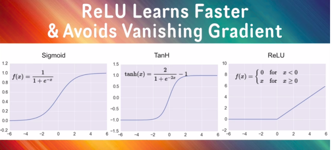
It is actually done with the Sigmoid Functions. Sigmoid Functions are simplest possible functions goes between 0 and 1. As I said in my previous blog, the sigmoid functions behave like a human brain. Middle layers between the top to the end except the final output are applied Sigmoid Functions and the output is applied Softmax function. So this is the mathematical way of implementing multilayered or convolutional neural networks.
In TensorFlow it can be implemented like this,
X  = tf.reshape(X, [-1, 28*28])
Y1 = tf.nn.Sigmoid(tf.matmul(X, W1) + b1)
Y2 = tf.nn.Sigmoid(tf.matmul(Y1, W2) + b2)
Y3 = tf.nn.Sigmoid(tf.matmul(Y2, W3) + b3)
Y4 = tf.nn.Sigmoid(tf.matmul(Y3, W4) + b4)
Y  = tf.nn.Sigmoid(tf.matmul(Y4, W5) + b5)
This step alone does not give the feasible output, but the accuracy will really shoot up slowly in some time interval. In order to shoot up the Accuracy quickly, we just change the activation function from Sigmoid to RELU.
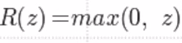
Rectified Linear Unit(RELU):
The RELU is one of the new activation functions, which actually outputs zero to negative values and goes steeply to the peak for the positive results we obtain with our model. In deep learning, RELU is the best choice for the activation function which avoids the Vanishing Gradient problem.
Y = tf.nn.relu(tf.matmul(X, W) + b)
So after applying RELU function, the accuracy will be improved. If it does not have any effect on the system it needs to be undergone Regularization. The popular regularization method is Dropout which actually makes some neurons picked randomly to zero. Is that really helpful? Yes, it will.
pkeep = tf.placeholder(tf.float32)
Yf = tf.nn.relu(tf.matmul(X, W) + b)
Y = tf.nn.dropout(Yf, pkeep)
The following table gives an overview of what the Martin Garner, gave in the tutorial,
| S.No | Network | Result |
|---|---|---|
| 1. | 5 layered Neural Network with Sigmoid |
97.9 % |
| 2. | 5 Layered RELU network Learning Rate Decay (0.003 i.e 300 iterations) |
98.2 % Peak(More Volatility) |
| 3. | RELU with Learning Rate Decay 0.0001(10,000 iterations) |
98.2 % Sustained |
| 4. | RELU with LRD 0.0001 and Dropout 0.75 |
Over-fitting comes down |
